3. Neon

In this section we explore Neon, ARM’s advanced SIMD (Single Instruction, Multiple Data) architecture extension. Our goal is to understand how to implement Neon kernels and how to optimize them for maximum performance.

3.1 Execution Throughput and Latency

The first task was to benchmark the execution throughput and latency of some selected FP32 Neon instructions. Specifically, we were looking at:

1. FMLA (vector) instruction

2. FMADD (scalar) instruction

3.1.1 Throughput

To analyze the throughput, we compared the performance of the following variants:

1. FMLA (vector) with arrangement specifier 4S

2. FMLA (vector) with arrangement specifier 2S

3. FMADD (scalar), single-precision variant

To compare the throughput of these variants, we created an assembly program for each of them. To ensure instruction-level parallelism, we carefully designed the inner loops of these programs to avoid register dependencies between successive instructions. The calculations and loop structures we used are shown here:

FMLA (vector) with arrangement specifier 4S

loop:
    .rept 100
    fmla  v0.4s,  v8.4s, v16.4s
    fmla  v1.4s,  v9.4s, v17.4s
    fmla  v2.4s, v10.4s, v18.4s
    fmla  v3.4s, v11.4s, v19.4s
    fmla  v4.4s, v12.4s, v20.4s

    fmla  v5.4s, v13.4s, v21.4s
    fmla  v6.4s, v14.4s, v22.4s
    fmla  v7.4s, v15.4s, v23.4s
    fmla  v8.4s, v16.4s, v24.4s
    fmla  v9.4s, v17.4s, v25.4s

    fmla v10.4s, v18.4s, v26.4s
    fmla v11.4s, v19.4s, v27.4s
    fmla v12.4s, v20.4s, v28.4s
    fmla v13.4s, v21.4s, v29.4s
    fmla v14.4s, v22.4s, v30.4s

    fmla v15.4s, v23.4s, v31.4s
    fmla v16.4s, v24.4s,  v0.4s
    fmla v17.4s, v25.4s,  v1.4s
    fmla v18.4s, v26.4s,  v2.4s
    fmla v19.4s, v27.4s,  v3.4s

    fmla v20.4s, v28.4s,  v4.4s
    fmla v21.4s, v29.4s,  v5.4s
    fmla v22.4s, v30.4s,  v6.4s
    fmla v23.4s, v31.4s,  v7.4s
    fmla v24.4s,  v0.4s,  v8.4s

    fmla v25.4s,  v1.4s,  v9.4s
    fmla v26.4s,  v2.4s, v10.4s
    fmla v27.4s,  v3.4s, v11.4s
    fmla v28.4s,  v4.4s, v12.4s
    fmla v29.4s,  v5.4s, v13.4s

    fmla v30.4s,  v6.4s, v14.4s
    fmla v31.4s,  v7.4s, v15.4s
    .endr

FMLA (vector) with arrangement specifier 2S

loop:
    .rept 100
    fmla  v0.2s,  v8.2s, v16.2s
    fmla  v1.2s,  v9.2s, v17.2s
    fmla  v2.2s, v10.2s, v18.2s
    fmla  v3.2s, v11.2s, v19.2s
    fmla  v4.2s, v12.2s, v20.2s

    fmla  v5.2s, v13.2s, v21.2s
    fmla  v6.2s, v12.2s, v22.2s
    fmla  v7.2s, v15.2s, v23.2s
    fmla  v8.2s, v16.2s, v24.2s
    fmla  v9.2s, v17.2s, v25.2s

    fmla v10.2s, v18.2s, v26.2s
    fmla v11.2s, v19.2s, v27.2s
    fmla v12.2s, v20.2s, v28.2s
    fmla v13.2s, v21.2s, v29.2s
    fmla v12.2s, v22.2s, v30.2s

    fmla v15.2s, v23.2s, v31.2s
    fmla v16.2s, v24.2s,  v0.2s
    fmla v17.2s, v25.2s,  v1.2s
    fmla v18.2s, v26.2s,  v2.2s
    fmla v19.2s, v27.2s,  v3.2s

    fmla v20.2s, v28.2s,  v4.2s
    fmla v21.2s, v29.2s,  v5.2s
    fmla v22.2s, v30.2s,  v6.2s
    fmla v23.2s, v31.2s,  v7.2s
    fmla v24.2s,  v0.2s,  v8.2s

    fmla v25.2s,  v1.2s,  v9.2s
    fmla v26.2s,  v2.2s, v10.2s
    fmla v27.2s,  v3.2s, v11.2s
    fmla v28.2s,  v4.2s, v12.2s
    fmla v29.2s,  v5.2s, v13.2s

    fmla v30.2s,  v6.2s, v12.2s
    fmla v31.2s,  v7.2s, v15.2s
    .endr

FMADD (scalar), single-precision variant

loop:
    .rept 100
    fmadd  s0,  s8, s16, s24
    fmadd  s1,  s9, s17, s25
    fmadd  s2, s10, s18, s26
    fmadd  s3, s11, s19, s27
    fmadd  s4, s12, s20, s28

    fmadd  s5, s13, s21, s29
    fmadd  s6, s14, s22, s30
    fmadd  s7, s15, s23, s31
    fmadd  s8, s16, s24, s0
    fmadd  s9, s17, s25, s1

    fmadd s10, s18, s26, s2
    fmadd s11, s19, s27, s3
    fmadd s12, s20, s28, s4
    fmadd s13, s21, s29, s5
    fmadd s14, s22, s30, s6

    fmadd s15, s23, s31, s7
    fmadd s16, s24,  s0, s8
    fmadd s17, s25,  s1, s9
    fmadd s18, s26,  s2, s10
    fmadd s19, s27,  s3, s11

    fmadd s20, s28,  s4, s12
    fmadd s21, s29,  s5, s13
    fmadd s22, s30,  s6, s14
    fmadd s23, s31,  s7, s15
    fmadd s24,  s0,  s8, s16

    fmadd s25,  s1,  s9, s17
    fmadd s26,  s2, s10, s18
    fmadd s27,  s3, s11, s19
    fmadd s28,  s4, s12, s20
    fmadd s29,  s5, s13, s21

    fmadd s30,  s6, s14, s22
    fmadd s31,  s7, s15, s23
    .endr

    subs x0, x0, #1
    b.gt loop

We then implemented a C++ microbenchmark to evaluate each version. For each function, we:

1. Performed a warm-up

2. Measured the execution time

3. Counted the number of operations

4. Calculated the resulting GFLOPs

Example benchmark for FMLA 4S

        // Warmup
        fmla_4s_instr( 100, g_4s_registers );

        auto l_start_time = std::chrono::high_resolution_clock::now();
        fmla_4s_instr( n, g_4s_registers );
        auto l_end_time = std::chrono::high_resolution_clock::now();
        elapsedTime = std::chrono::duration_cast<std::chrono::microseconds>( l_end_time - l_start_time ).count() / 1e6;

        // per FMLA: 4 Muls, 4 Adds
        // 32 fmla
        // rept 100
        // n: loop iterations
        totalOps = (2 * 4) * 32 * 100 * n;

Calculations for 2S and FMADD (scalar):

Calculations for FMLA 2S

        // per FMLA: 2 Muls, 2 Adds
        // 32 fmla
        // rept 100
        // n: loop iterations
        totalOps = (2 * 2) * 32 * 100 * n;

Calculations for FMADD

        // per FMADD: 1 Mul, 1 Add
        // 32 fmadd
        // rept 100
        // n: loop iterations
        totalOps = (2 * 1) * 32 * 100 * n;

The measured throughput results we obtained were as follows:

Measured Throughput Results

Benchmarking FMLA 4s throughput ...
-----------------------------------------------
Measuring throughput for FMLA_4sInstruction
Total time (s):   1.96706
Instructions per Second:   1.30144e+11
Estimated GOPS:   130.144 GFLOPs/sec
-----------------------------------------------

Benchmarking FMLA 2s throughput ...
-----------------------------------------------
Measuring throughput for FMLA_2sInstruction
Total time (s):   2.53647
Instructions per Second:   5.04638e+10
Estimated GOPS:   50.4638 GFLOPs/sec
-----------------------------------------------

Benchmarking FMADD throughput ...
-----------------------------------------------
Measuring throughput for FMADDInstruction
Total time (s):   3.52918
Instructions per Second:   1.81345e+10
Estimated GOPS:   18.1345 GFLOPs/sec
-----------------------------------------------

We observe that:

• FMLA 4S achieves approximately 2.5 times the performance of FMLA 2S

• FMLA 2S similarly outperforms FMADD (scalar) by a factor of 2.5

These results highlight the benefit of data-level parallelism through vector operations. The higher the vector width, the more operations are performed per instruction, therefore resulting in a significantly improved throughput compared to a scalar execution.

3.1.2 Latency

To analyze the execution latency of the FMLA vector instruction with arrangement specifier 4S, we considered two dependency scenarios:

1. Each instruction depends on the destination register and one source register of the previous instruction.

FMLA instructions with dependencies on the destination and one source registers

    fmla v0.4s, v0.4s,  v1.4s
    fmla v0.4s, v0.4s,  v2.4s
    fmla v0.4s, v0.4s,  v3.4s
    fmla v0.4s, v0.4s,  v4.4s

2. Each instruction depends only on the destination register of the previous instruction

FMLA instructions with dependency only on the destination register

    fmla v0.4s,  v1.4s,  v9.4s
    fmla v0.4s,  v2.4s, v10.4s
    fmla v0.4s,  v3.4s, v11.4s
    fmla v0.4s,  v4.4s, v12.4s

In both cases, 32 dependent FMLA instructions were executed in a loop, repeated 100 times. The results for both cases are shown below:

Latency benchmark results for the two dependency scenarios

Benchmarking FMLA 4s source register latency ...
-----------------------------------------------
Measuring latency for FMLA_SourceInstruction
Total time (s):   3.30277
Instructions per Second:   1.16266e+10
Estimated GOPS:   11.6266 GFLOPs/sec
-----------------------------------------------

Benchmarking FMLA 4s destination register latency ...
-----------------------------------------------
Measuring latency for FMLA_DestinationInstruction
Total time (s):   3.30207
Instructions per Second:   1.16291e+10
Estimated GOPS:   11.6291 GFLOPs/sec
-----------------------------------------------

We observed that both scenarios produced nearly identical performance results. Therefore, we focused our latency calculations only on the first scenario.

From our measurement, we got \(1.16266 \times 10^{10}\) instructions per second. This yields a per-instruction latency of approximately \(\frac{1}{1.16266 \times 10^{10}} \approx 8.6 \times 10^{-11}\) seconds. Assuming a clock frequency of 4.4 GHz, we estimated the latency in clock cycles as \(8.6 \times 10^{-11} \times 4.4 \times 10^9 = 0.3784\) cycles.

This value suggests that the latency of a single FMLA 4S instruction is well below one clock cycle.

3.2 Microkernel

For the second task, we implemented a Neon-based microkernel to perform a matrix-matrix multiplication with the following dimensions:

1. Matrix A: 16 x 1

2. Matrix B: 1 x 6

3. Matrix C: 16 x 6

For the task we were provided with the following C function signature:

Function Signature

/**
 * @brief GEMM that computes: C+=AB.
 * @param a    Pointer to column-major matrix A.
 * @param b    Pointer to column-major matrix B.
 * @param c    Pointer to column-major matrix C.
 * @param ld_a Leading dimension of A.
 * @param ld_b Leading dimension of B.
 * @param ld_c Leading dimension of C.
 **/
void matmul_16_6_1( float   const * a,
                    float   const * b,
                    float         * c,
                    int64_t         ld_a,
                    int64_t         ld_b,
                    int64_t         ld_c );

3.2.1 Neon Microkernel

We developed three different versions of this microkernel. With each version, we wanted to compare different data-loading, register usage and data reuse strategies:

The first version:

1. Load the entire Matrix A (16 x 1)

2. Load three individual elements (1 x 1) of Matrix B

3. Load the entire Matrix C (16 x 6)

b1_matmul_16_6_1.s

/*
 * Load 3 elements of B
 */
mov x6, x1              // current column of B

ldr s28, [x6]           // Column B(0)
add x6, x6, x4

ldr s29, [x6]           // Column B(1)
add x6, x6, x4

ldr s30, [x6]           // Column B(2)
add x6, x6, x4

/*
 * Multiply and accumulate (1 / 2)
 */
fmla v4.4s, v0.4s, v28.s[0]
fmla v5.4s, v1.4s, v28.s[0]
fmla v6.4s, v2.4s, v28.s[0]
fmla v7.4s, v3.4s, v28.s[0]

fmla v8.4s,  v0.4s, v29.s[0]
fmla v9.4s,  v1.4s, v29.s[0]
fmla v10.4s, v2.4s, v29.s[0]
fmla v11.4s, v3.4s, v29.s[0]

fmla v12.4s, v0.4s, v30.s[0]
fmla v13.4s, v1.4s, v30.s[0]
fmla v14.4s, v2.4s, v30.s[0]
fmla v15.4s, v3.4s, v30.s[0]

The second version:

1. Load the entire Matrix A (16 x 1)

2. Load one element of Matrix B

3. Load the entire Matrix C (16 x 6)

b2_matmul_16_6_1.s

/*
 * Load column of B (1 / 6)
 */
mov x6, x1              // current column of B

ldr s28, [x6]           // Column B(0)
add x6, x6, x4

/*
 * Multiply and accumulate (1 / 6)
 */
fmla v4.4s, v0.4s, v28.s[0]
fmla v5.4s, v1.4s, v28.s[0]
fmla v6.4s, v2.4s, v28.s[0]
fmla v7.4s, v3.4s, v28.s[0]

The third version:

1. Load the entire Matrix A (16 x 1)

2. Load one column of Matrix B

3. Load one column of Matrix C (16 x 1)

b3_matmul_16_6_1.s

/*
 * Matrix C: Column 0
 */
// Load column of B
ldr s8, [x6]

// Load column of C
ldp q4, q5, [x7]
ldp q6, q7, [x7, #32]

// Multiply and accumulate
fmla v4.4s, v0.4s, v8.s[0]
fmla v5.4s, v1.4s, v8.s[0]
fmla v6.4s, v2.4s, v8.s[0]
fmla v7.4s, v3.4s, v8.s[0]

// Store column of C
stp q4, q5, [x7]
stp q6, q7, [x7, #32]

3.2.2 Testing and Benchmarking

To validate and compare our implementations, we took the following steps:

1. We developed a basic kernel driver to inspect our output correctness visually

2. We used Catch2 to verify the correctness of our implementations

3. We implemented a benchmark to measure GFLOPs for all three versions

The GFLOPs were calculated with the following formula:

GFLOPs calculation

double totalOps = ( 6 * 16 ) * 2;
double opsPerIteration = totalOps * loopIterations;

double opsPerSec = opsPerIteration / elapsedTime;
double gflops = opsPerIteration / ( elapsedTime * 1e9 );

Each kernel was executed with 50,000 warmup iterations to reduce variability and ensure fair comparisons. The benchmark produced the following performance results:

GFLOPs results for all three versions

Benchmarking V1 Matmul throughput ...
-----------------------------------------------
Measuring throughput for Instruction
Total time (s):   2.93595
Instructions per Second:   3.26981e+10
Estimated GFLOPS:   32.6981 GFLOPS/sec
-----------------------------------------------

Benchmarking V2 Matmul throughput ...
-----------------------------------------------
Measuring throughput for Instruction
Total time (s):   2.90291
Instructions per Second:   3.30702e+10
Estimated GFLOPS:   33.0702 GFLOPS/sec
-----------------------------------------------

Benchmarking V3 Matmul throughput ...
-----------------------------------------------
Measuring throughput for Instruction
Total time (s):   2.79132
Instructions per Second:   3.43923e+10
Estimated GFLOPS:   34.3923 GFLOPS/sec
-----------------------------------------------

The results show that performance improved incrementally with each version. The best-performing kernel outperformed the least-performing by approximately 1.7 GFLOPs, highlighting the importance of careful memory and register management.

Note

Even though the third implementation achieved the best performance, it is tailored specifically to the given matrix dimensions. As the K dimension increases, the kernel would repeatedly reload columns of matrix C, leading to significant performance degradation.

3.3 Loops

After implementing and benchmarking our initial 16x6x1 Neon microkernel, the next step was to scale this kernel for the use with larger matrices. To achieve this, we extended the kernel along the three matrix dimensions K, M, and N, by introducing loops around our base kernel.

3.3.1 Loop Implementations

Our first step was to handle larger K dimensions. Therefore, we transformed our kernel into a 16x6x64 kernel. The core of the microkernel remained mostly unchanged, except that we updated the input pointers for matrices A and B in each iteration:

• A is advanced by the given stride to move to the next column.

• B is advanced row-by-row, with a 4-byte step for each 32-bit float value.

The updated loop body is shown below:

Looping the matmul_16_6_1 kernel over the K dimension

    //  K loop counter
    mov x6, #64
    // set start of A
    mov x7, x0
    // set start of B
    mov x8, x1
    // init row count of B
    mov x9, #0

_k_loop:
    // load column of A
    ldp q24, q25, [x7] // 4 + 4 values
    ldp q26, q27, [x7, #32] // 4 + 4 values

    // B: COLUMN 0
    ldr s29, [x8]
    fmla v0.4s, v24.4s, v29.s[0]
    fmla v1.4s, v25.4s, v29.s[0]
    fmla v2.4s, v26.4s, v29.s[0]
    fmla v3.4s, v27.4s, v29.s[0]
    // B: COLUMN 1
    add x8, x8, x4
    ldr s29, [x8]
    fmla v4.4s, v24.4s, v29.s[0]
    fmla v5.4s, v25.4s, v29.s[0]
    fmla v6.4s, v26.4s, v29.s[0]
    fmla v7.4s, v27.4s, v29.s[0]
    // B: COLUMN 2
    add x8, x8, x4
    ldr s29, [x8]
    fmla  v8.4s, v24.4s, v29.s[0]
    fmla  v9.4s, v25.4s, v29.s[0]
    fmla v10.4s, v26.4s, v29.s[0]
    fmla v11.4s, v27.4s, v29.s[0]
    // B: COLUMN 3
    add x8, x8, x4
    ldr s29, [x8]
    fmla v12.4s, v24.4s, v29.s[0]
    fmla v13.4s, v25.4s, v29.s[0]
    fmla v14.4s, v26.4s, v29.s[0]
    fmla v15.4s, v27.4s, v29.s[0]
    // B: COLUMN 4
    add x8, x8, x4
    ldr s29, [x8]
    fmla v16.4s, v24.4s, v29.s[0]
    fmla v17.4s, v25.4s, v29.s[0]
    fmla v18.4s, v26.4s, v29.s[0]
    fmla v19.4s, v27.4s, v29.s[0]
    // B: COLUMN 5
    add x8, x8, x4
    ldr s29, [x8]
    fmla v20.4s, v24.4s, v29.s[0]
    fmla v21.4s, v25.4s, v29.s[0]
    fmla v22.4s, v26.4s, v29.s[0]
    fmla v23.4s, v27.4s, v29.s[0]

    // move to next column of A
    add x7, x7, x3
    // move to next row of B
    mov x8, x1
    add x9, x9, #4
    add x8, x8, x9

    // decrement loop counter
    sub x6, x6, #1
    // check if loop counter is zero
    cbnz x6, _k_loop

The matmul_16_6_1 kernel mostly stayed the same, except that for each K loop, we now need to adjust the pointers to the input matrices A and B. At the end of each loop, we move the pointers to A to the next column by adding the given stride. In B, we need to move the pointer to the next row. Therefore, we jump by 4 Bytes (since we are using 32-bit floats) from the starting address of B. To keep jumping to the next row in each loop, we accumulate the offset of 4 Bytes in the register x9.

In the second step we added a loop over the M dimension to build a 64x6x64 kernel. In this version, we reused the kernel for processing 16 rows of M at a time and iterated four times to cover all 64 rows. That means, at the end of the M loop, we advance the pointers of A and C to the next block.

First part of looping over the M dimension

    // save base matrix pointers
    mov x7, x0 // A
    mov x8, x1 // B
    mov x9, x2 // C

    // M loop counter
    mov x11, #4 // 64/16 = 4 blocks

_m_loop:
// ------------------------------------------
// START matmul_16_6_64
// ------------------------------------------

    // LOAD MATRIX C
    mov x12, x9
    // first column
    ldp q0, q1, [x12]
    ldp q2, q3, [x12, #32]
    // second column
    add x12, x12, x5
    ldp q4, q5, [x12]
    ldp q6, q7, [x12, #32]
    // third column
    add x12, x12, x5
    ldp q8, q9, [x12]
    ldp q10, q11, [x12, #32]
    // fourth column
    add x12, x12, x5
    ldp q12, q13, [x12]
    ldp q14, q15, [x12, #32]
    // fifth column
    add x12, x12, x5
    ldp q16, q17, [x12]
    ldp q18, q19, [x12, #32]
    // sixth column
    add x12, x12, x5
    ldp q20, q21, [x12]
    ldp q22, q23, [x12, #32]

    // K loop counter
    mov x14, #64
    // set start of A
    mov x15, x7
    // set start of B
    mov x16, x8
    // init row count of B
    mov x17, #0
_k_loop:

Second part of looping over the M dimension

    // check if loop counter is zero
    cbnz x14, _k_loop

    // STORE MATRIX C
    mov x12, x9
    // first column
    stp q0, q1, [x12]
    stp q2, q3, [x12, #32]
    // second column
    add x12, x12, x5
    stp q4, q5, [x12]
    stp q6, q7, [x12, #32]
    // third column
    add x12, x12, x5
    stp q8, q9, [x12]
    stp q10, q11, [x12, #32]
    // fourth column
    add x12, x12, x5
    stp q12, q13, [x12]
    stp q14, q15, [x12, #32]
    // fifth column
    add x12, x12, x5
    stp q16, q17, [x12]
    stp q18, q19, [x12, #32]
    // sixth column
    add x12, x12, x5
    stp q20, q21, [x12]
    stp q22, q23, [x12, #32]

// ------------------------------------------
// END matmul_16_6_64
// ------------------------------------------

    // increase A and C pointers for next block
    add x7, x7, #16*4
    add x9, x9, #16*4

    // decrement m loop counter
    sub x11, x11, #1
    // check if loop counter is zero
    cbnz x11, _m_loop

The third step was to implement a loop in the N dimension, extending the kernel to handle a 64x48x64 matrix multiplication. This required dividing N into 8 blocks of 6 columns, resulting in 8 loop iterations. For each N loop, it is important to first reset the pointer of A to the original address. After each iteration, we need to move the pointers of B and C to the next block:

First part of looping over the N dimension

    // set base matrix pointers
    mov x20, x1 // B
    mov x21, x2 // C

    // N loop counter
    mov x19, #8 // 48/6 = 8 blocks

_n_loop:

    // M loop counter
    mov x11, #4 // 64/16 = 4 blocks

    // set matrix pointers
    mov x7, x0 // A
    mov x8, x20 // B
    mov x9, x21 // C

_m_loop:

Second part of looping over the N dimension

    // decrement m loop counter
    sub x11, x11, #1
    // check if loop counter is zero
    cbnz x11, _m_loop
// END M LOOP

    // increase B and C pointers for next block
    // (jump 6 columns) 6*x4, 6*x5
    add x20, x20, x22
    add x21, x21, x23

    // decrement n loop counter
    sub x19, x19, #1
    // check if loop counter is zero
    cbnz x19, _n_loop
// END N LOOP

3.3.2 Testing and Benchmarking

To ensure correctness, we wrote unit tests for all three of our kernels. To execute the tests, we need to step in the correct directory (src/submissions/03_neon/03_loops) and compile the code by invoking make. This will create an executable that can be run with ./build/test.

We also benchmarked each kernel to measure their performance in GFLOPs, using the standard formula:

\[M \cdot N \cdot K \cdot \text{Ops Per FMLA}\]

The benchmarking results that we obtained are:

GFLOPs calculations for the MatMul kernels

Benchmarking Matmul_16_6_64 throughput ...
-----------------------------------------------
Measuring throughput for Instruction
Total time (s):   1.89248
Instructions per Second:   1.29861e+11
Estimated GFLOPS:   129.861 GFLOPS/sec
-----------------------------------------------

Benchmarking Matmul_64_6_64 Matmul throughput ...
-----------------------------------------------
Measuring throughput for Instruction
Total time (s):   1.84635
Instructions per Second:   1.33106e+11
Estimated GFLOPS:   133.106 GFLOPS/sec
-----------------------------------------------

Benchmarking Matmul_64_48_64 Matmul throughput ...
-----------------------------------------------
Measuring throughput for Instruction
Total time (s):   1.49743
Instructions per Second:   1.31297e+11
Estimated GFLOPS:   131.297 GFLOPS/sec
-----------------------------------------------

Our results indicate that the number of GFLOPs is very consistent, even when scaling the size of our matrices.

3.4 SIMD Lanes

In this task, our goal was to implement two kernels capable of handling cases where the M dimension is not a multiple of 4. Specifically, we focused on the following matrix shapes:

1. the M=14, N=6 and K=64, and

2. the M=15, N=6 and K=64

3.4.1 Matmul_14_6_64

For the case M=14, we explored four different implementations:

In our first approach we used two loops. The first loop computes a 12 x 64 block of matrix C, while the second loop handles the remaining 2 x 64 block.

Second loop for the 2 x 64 matrix calculation

_k2_loop:
    // load column of A
    ldr d24, [x7]   // 2 values

    // B: COLUMN 0
    ldr s29, [x8]
    fmla v3.2s, v24.2s, v29.s[0]

    // B: COLUMN 1
    add x8, x8, x4
    ldr s29, [x8]
    fmla v7.2s, v24.2s, v29.s[0]

    // B: COLUMN 2
    add x8, x8, x4
    ldr s29, [x8]
    fmla v11.2s, v24.2s, v29.s[0]

    // B: COLUMN 3
    add x8, x8, x4
    ldr s29, [x8]
    fmla v15.2s, v24.2s, v29.s[0]

    // B: COLUMN 4
    add x8, x8, x4
    ldr s29, [x8]
    fmla v19.2s, v24.2s, v29.s[0]
    
    // B: COLUMN 5
    add x8, x8, x4
    ldr s29, [x8]
    fmla v23.2s, v24.2s, v29.s[0]

    // move to next column of A
    add x7, x7, x3
    // move to next row of B
    mov x8, x1
    add x9, x9, #4
    add x8, x8, x9

    // decrement loop counter
    sub x6, x6, #1
    // check if loop counter is zero
    cbnz x6, _k2_loop

For our second approach we used a single loop. Here, we load the entire matrix C and process each column of A in a loop iteration using three FMLA (4s) instructions and one FMLA (2s) instruction.

Calculating matrix C with a single loop using different calculations

_k1_loop:
    // load column of A
    ldp q24, q25, [x7] // 4 + 4 values
    ldr q26, [x7, #32] // 4 values
    ldr d27, [x7, #48] // 2 values

    // B: COLUMN 0
    ldr s29, [x8]
    fmla v0.4s, v24.4s, v29.s[0]
    fmla v1.4s, v25.4s, v29.s[0]
    fmla v2.4s, v26.4s, v29.s[0]
    fmla v3.2s, v27.2s, v29.s[0]
    // B: COLUMN 1
    add x8, x8, x4
    ldr s29, [x8]
    fmla v4.4s, v24.4s, v29.s[0]
    fmla v5.4s, v25.4s, v29.s[0]
    fmla v6.4s, v26.4s, v29.s[0]
    fmla v7.2s, v27.2s, v29.s[0]
    // B: COLUMN 2
    add x8, x8, x4
    ldr s29, [x8]
    fmla  v8.4s, v24.4s, v29.s[0]
    fmla  v9.4s, v25.4s, v29.s[0]
    fmla v10.4s, v26.4s, v29.s[0]
    fmla v11.2s, v27.2s, v29.s[0]
    // B: COLUMN 3
    add x8, x8, x4
    ldr s29, [x8]
    fmla v12.4s, v24.4s, v29.s[0]
    fmla v13.4s, v25.4s, v29.s[0]
    fmla v14.4s, v26.4s, v29.s[0]
    fmla v15.2s, v27.2s, v29.s[0]
    // B: COLUMN 4
    add x8, x8, x4
    ldr s29, [x8]
    fmla v16.4s, v24.4s, v29.s[0]
    fmla v17.4s, v25.4s, v29.s[0]
    fmla v18.4s, v26.4s, v29.s[0]
    fmla v19.2s, v27.2s, v29.s[0]
    // B: COLUMN 5
    add x8, x8, x4
    ldr s29, [x8]
    fmla v20.4s, v24.4s, v29.s[0]
    fmla v21.4s, v25.4s, v29.s[0]
    fmla v22.4s, v26.4s, v29.s[0]
    fmla v23.2s, v27.2s, v29.s[0]

    // move to next column of A
    add x7, x7, x3
    // move to next row of B
    mov x8, x1
    add x9, x9, #4
    add x8, x8, x9

    // decrement loop counter
    sub x6, x6, #1
    // check if loop counter is zero
    cbnz x6, _k1_loop

In our third approach we were also using the single loop version, but this time we padded a register of A, that holds the remaining two values with two zero values using mov v27.s[2], wzr and mov v27.s[3], wzr. This allows us to use four FMLA (4s) instructions.

Using zero-padding to use four FMLA (4s) instructions

_k1_loop:
    // load column of A
    ldp q24, q25, [x7] // 4 + 4 values
    ldr q26, [x7, #32] // 4 values
    ldr d27, [x7, #48] // 2 values
    mov v27.s[2], wzr
    mov v27.s[3], wzr

    // B: COLUMN 0
    ldr s29, [x8]
    
    fmla v0.4s, v24.4s, v29.s[0]
    fmla v1.4s, v25.4s, v29.s[0]
    fmla v2.4s, v26.4s, v29.s[0]
    fmla v3.4s, v27.4s, v29.s[0]
    // B: COLUMN 1
    add x8, x8, x4
    ldr s29, [x8]
    fmla v4.4s, v24.4s, v29.s[0]
    fmla v5.4s, v25.4s, v29.s[0]
    fmla v6.4s, v26.4s, v29.s[0]
    fmla v7.4s, v27.4s, v29.s[0]
    // B: COLUMN 2
    add x8, x8, x4
    ldr s29, [x8]
    fmla  v8.4s, v24.4s, v29.s[0]
    fmla  v9.4s, v25.4s, v29.s[0]
    fmla v10.4s, v26.4s, v29.s[0]
    fmla v11.4s, v27.4s, v29.s[0]
    // B: COLUMN 3
    add x8, x8, x4
    ldr s29, [x8]
    fmla v12.4s, v24.4s, v29.s[0]
    fmla v13.4s, v25.4s, v29.s[0]
    fmla v14.4s, v26.4s, v29.s[0]
    fmla v15.4s, v27.4s, v29.s[0]
    // B: COLUMN 4
    add x8, x8, x4
    ldr s29, [x8]
    fmla v16.4s, v24.4s, v29.s[0]
    fmla v17.4s, v25.4s, v29.s[0]
    fmla v18.4s, v26.4s, v29.s[0]
    fmla v19.4s, v27.4s, v29.s[0]
    // B: COLUMN 5
    add x8, x8, x4
    ldr s29, [x8]
    fmla v20.4s, v24.4s, v29.s[0]
    fmla v21.4s, v25.4s, v29.s[0]
    fmla v22.4s, v26.4s, v29.s[0]
    fmla v23.4s, v27.4s, v29.s[0]

    // move to next column of A
    add x7, x7, x3
    // move to next row of B
    mov x8, x1
    add x9, x9, #4
    add x8, x8, x9

    // decrement loop counter
    sub x6, x6, #1
    // check if loop counter is zero
    cbnz x6, _k1_loop

In our fourth approach we simply copied the second version and changed our loads for matrix A and C. We used ld1 instead of ldp.

Single loop version using ld1 loads

_k1_loop:
    // load column of A
    ld1 {v24.4s-v27.4s}, [x7]
    ldr d27, [x7, #48] // 2 values

    // B: COLUMN 0
    ldr s29, [x8]
    fmla v0.4s, v24.4s, v29.s[0]
    fmla v1.4s, v25.4s, v29.s[0]
    fmla v2.4s, v26.4s, v29.s[0]
    fmla v3.2s, v27.2s, v29.s[0]
    // B: COLUMN 1
    add x8, x8, x4
    ldr s29, [x8]
    fmla v4.4s, v24.4s, v29.s[0]
    fmla v5.4s, v25.4s, v29.s[0]
    fmla v6.4s, v26.4s, v29.s[0]
    fmla v7.2s, v27.2s, v29.s[0]
    // B: COLUMN 2
    add x8, x8, x4
    ldr s29, [x8]
    fmla  v8.4s, v24.4s, v29.s[0]
    fmla  v9.4s, v25.4s, v29.s[0]
    fmla v10.4s, v26.4s, v29.s[0]
    fmla v11.2s, v27.2s, v29.s[0]
    // B: COLUMN 3
    add x8, x8, x4
    ldr s29, [x8]
    fmla v12.4s, v24.4s, v29.s[0]
    fmla v13.4s, v25.4s, v29.s[0]
    fmla v14.4s, v26.4s, v29.s[0]
    fmla v15.2s, v27.2s, v29.s[0]
    // B: COLUMN 4
    add x8, x8, x4
    ldr s29, [x8]
    fmla v16.4s, v24.4s, v29.s[0]
    fmla v17.4s, v25.4s, v29.s[0]
    fmla v18.4s, v26.4s, v29.s[0]
    fmla v19.2s, v27.2s, v29.s[0]
    // B: COLUMN 5
    add x8, x8, x4
    ldr s29, [x8]
    fmla v20.4s, v24.4s, v29.s[0]
    fmla v21.4s, v25.4s, v29.s[0]
    fmla v22.4s, v26.4s, v29.s[0]
    fmla v23.2s, v27.2s, v29.s[0]

    // move to next column of A
    add x7, x7, x3
    // move to next row of B
    mov x8, x1
    add x9, x9, #4
    add x8, x8, x9

    // decrement loop counter
    sub x6, x6, #1
    // check if loop counter is zero
    cbnz x6, _k1_loop

To compare our different versions, we performed benchmarks on each kernel. Our benchmarking results are as follows:

Benchmarking results for matmul_14_6_64 approaches

Benchmarking V1_Matmul_14_6_64 throughput ...
-----------------------------------------------
Measuring throughput for Instruction
Total time (s):   2.46349
Instructions per Second:   8.72907e+10
Estimated GFLOPS:   87.2907 GFLOPS/sec
-----------------------------------------------

Benchmarking V2_Matmul_14_6_64 throughput ...
-----------------------------------------------
Measuring throughput for Instruction
Total time (s):   1.86679
Instructions per Second:   1.15192e+11
Estimated GFLOPS:   115.192 GFLOPS/sec
-----------------------------------------------

Benchmarking V3_Matmul_14_6_64 throughput ...
-----------------------------------------------
Measuring throughput for Instruction
Total time (s):   2.06673
Instructions per Second:   1.04048e+11
Estimated GFLOPS:   104.048 GFLOPS/sec
-----------------------------------------------

Benchmarking V4_Matmul_14_6_64 throughput ...
-----------------------------------------------
Measuring throughput for Instruction
Total time (s):   1.90053
Instructions per Second:   1.13147e+11
Estimated GFLOPS:   113.147 GFLOPS/sec
-----------------------------------------------

Our results indicate that the second version, using three FMLA (4s) instructions and one FMLA (2s) instruction, achieved the best performance. The version using ld1 loads achieved a similar GFLOPs.

3.4.2 Matmul_15_6_64

For the case M=15, we implemented and tested three kernels:

In our first approach we similarly to the M=14 case, split the computation into two loops. The first loop handles a 12 x 64 block, and the second loop processed the remaining 3 x 64 block of matrix C.

Second loop for the 3 x 64 matrix calculation

_k2_loop:
    // load column of A
    ldr d24, [x7]   // 2 values
    ldr s25, [x7, #8]

    // B: COLUMN 0
    ldr s29, [x8]
    fmla v0.2s, v24.2s, v29.s[0]
    fmadd s1, s25, s29, s1
    // B: COLUMN 1
    add x8, x8, x4
    ldr s29, [x8]
    fmla v2.2s, v24.2s, v29.s[0]
    fmadd s3, s25, s29, s3
    // B: COLUMN 2
    add x8, x8, x4
    ldr s29, [x8]
    fmla v4.2s, v24.2s, v29.s[0]
    fmadd s5, s25, s29, s5
    // B: COLUMN 3
    add x8, x8, x4
    ldr s29, [x8]
    fmla v6.2s, v24.2s, v29.s[0]
    fmadd s7, s25, s29, s7
    // B: COLUMN 4
    add x8, x8, x4
    ldr s29, [x8]
    fmla v8.2s, v24.2s, v29.s[0]
    fmadd s9, s25, s29, s9
    // B: COLUMN 5
    add x8, x8, x4
    ldr s29, [x8]
    fmla v10.2s, v24.2s, v29.s[0]
    fmadd s11, s25, s29, s11

    // move to next column of A
    add x7, x7, x3
    // move to next row of B
    mov x8, x1
    add x9, x9, #4
    add x8, x8, x9

    // decrement loop counter
    sub x6, x6, #1
    // check if loop counter is zero
    cbnz x6, _k2_loop

In the second approach we implement the kernel using a single loop. We load matrix A column-wise and calculate parts of matrix C using four FMLA (4s) instructions. We zeroed out the last element in the final vector register of matrix A with mov v27.s[3], wzr to safely operate on a full register.

Single loop version using ldp loads

_k1_loop:
    // load column of A
    ldp q24, q25, [x7] // 4 + 4 values
    ldr q26, [x7, #32] // 4 values
    ldr d27, [x7, #48] // 2 values
    ldr s28, [x7, #56] // 1 value

    mov v27.s[2], v28.s[0]
    mov v27.s[3], wzr

    // B: COLUMN 0
    ldr s29, [x8]
    
    fmla v0.4s, v24.4s, v29.s[0]
    fmla v1.4s, v25.4s, v29.s[0]
    fmla v2.4s, v26.4s, v29.s[0]
    fmla v3.4s, v27.4s, v29.s[0]
    // B: COLUMN 1
    add x8, x8, x4
    ldr s29, [x8]
    fmla v4.4s, v24.4s, v29.s[0]
    fmla v5.4s, v25.4s, v29.s[0]
    fmla v6.4s, v26.4s, v29.s[0]
    fmla v7.4s, v27.4s, v29.s[0]
    // B: COLUMN 2
    add x8, x8, x4
    ldr s29, [x8]
    fmla  v8.4s, v24.4s, v29.s[0]
    fmla  v9.4s, v25.4s, v29.s[0]
    fmla v10.4s, v26.4s, v29.s[0]
    fmla v11.4s, v27.4s, v29.s[0]
    // B: COLUMN 3
    add x8, x8, x4
    ldr s29, [x8]
    fmla v12.4s, v24.4s, v29.s[0]
    fmla v13.4s, v25.4s, v29.s[0]
    fmla v14.4s, v26.4s, v29.s[0]
    fmla v15.4s, v27.4s, v29.s[0]
    // B: COLUMN 4
    add x8, x8, x4
    ldr s29, [x8]
    fmla v16.4s, v24.4s, v29.s[0]
    fmla v17.4s, v25.4s, v29.s[0]
    fmla v18.4s, v26.4s, v29.s[0]
    fmla v19.4s, v27.4s, v29.s[0]
    // B: COLUMN 5
    add x8, x8, x4
    ldr s29, [x8]
    fmla v20.4s, v24.4s, v29.s[0]
    fmla v21.4s, v25.4s, v29.s[0]
    fmla v22.4s, v26.4s, v29.s[0]
    fmla v23.4s, v27.4s, v29.s[0]

    // move to next column of A
    add x7, x7, x3
    // move to next row of B
    mov x8, x1
    add x9, x9, #4
    add x8, x8, x9

    // decrement loop counter
    sub x6, x6, #1
    // check if loop counter is zero
    cbnz x6, _k1_loop

In the third approach we again changed the load instructions from ldp to ld1.

Single loop version using ld1 loads

_k1_loop:
    // load column of A
    ld1 {v24.4s-v26.4s}, [x7]  // 12 values
    ldr d27, [x7, #48]         // 2 values
    ldr s28, [x7, #56]         // 1 value

    mov v27.s[2], v28.s[0]
    mov v27.s[3], wzr

    // B: COLUMN 0
    ldr s29, [x8]
    
    fmla v0.4s, v24.4s, v29.s[0]
    fmla v1.4s, v25.4s, v29.s[0]
    fmla v2.4s, v26.4s, v29.s[0]
    fmla v3.4s, v27.4s, v29.s[0]
    // B: COLUMN 1
    add x8, x8, x4
    ldr s29, [x8]
    fmla v4.4s, v24.4s, v29.s[0]
    fmla v5.4s, v25.4s, v29.s[0]
    fmla v6.4s, v26.4s, v29.s[0]
    fmla v7.4s, v27.4s, v29.s[0]
    // B: COLUMN 2
    add x8, x8, x4
    ldr s29, [x8]
    fmla  v8.4s, v24.4s, v29.s[0]
    fmla  v9.4s, v25.4s, v29.s[0]
    fmla v10.4s, v26.4s, v29.s[0]
    fmla v11.4s, v27.4s, v29.s[0]
    // B: COLUMN 3
    add x8, x8, x4
    ldr s29, [x8]
    fmla v12.4s, v24.4s, v29.s[0]
    fmla v13.4s, v25.4s, v29.s[0]
    fmla v14.4s, v26.4s, v29.s[0]
    fmla v15.4s, v27.4s, v29.s[0]
    // B: COLUMN 4
    add x8, x8, x4
    ldr s29, [x8]
    fmla v16.4s, v24.4s, v29.s[0]
    fmla v17.4s, v25.4s, v29.s[0]
    fmla v18.4s, v26.4s, v29.s[0]
    fmla v19.4s, v27.4s, v29.s[0]
    // B: COLUMN 5
    add x8, x8, x4
    ldr s29, [x8]
    fmla v20.4s, v24.4s, v29.s[0]
    fmla v21.4s, v25.4s, v29.s[0]
    fmla v22.4s, v26.4s, v29.s[0]
    fmla v23.4s, v27.4s, v29.s[0]

    // move to next column of A
    add x7, x7, x3
    // move to next row of B
    mov x8, x1
    add x9, x9, #4
    add x8, x8, x9

    // decrement loop counter
    sub x6, x6, #1
    // check if loop counter is zero
    cbnz x6, _k1_loop

For these kernels we also executed benchmarks:

Benchmarking results for matmul_15_6_64 approaches

Benchmarking V1_Matmul_15_6_64 throughput ...
-----------------------------------------------
Measuring throughput for Instruction
Total time (s):   2.57834
Instructions per Second:   8.93599e+10
Estimated GFLOPS:   89.3599 GFLOPS/sec
-----------------------------------------------

Benchmarking V2_Matmul_15_6_64 throughput ...
-----------------------------------------------
Measuring throughput for Instruction
Total time (s):   2.1093
Instructions per Second:   1.09231e+11
Estimated GFLOPS:   109.231 GFLOPS/sec
-----------------------------------------------

Benchmarking V3_Matmul_15_6_64 throughput ...
-----------------------------------------------
Measuring throughput for Instruction
Total time (s):   2.10837
Instructions per Second:   1.09279e+11
Estimated GFLOPS:   109.279 GFLOPS/sec
-----------------------------------------------

Similar to the benchmarks for the matmul_14_6_64, the single loop approach significantly outperformed the two loop implementation. In this case, the difference was even bigger, with a gap of approximately 20 GFLOPs. However, unlike before, changing the load instruction from ldp to ld1 had no impact on the overall performance.

3.4.3 Generic Approach

As a proof of concept, we also implemented a generic matrix multiplication kernel capable of handling any M > 0. The core idea is to write specific kernels for M = 1, 2, ..., 8. For input sizes larger than M = 8, we then divide M by 8 (shift right by 3) and use that to loop the M = 8 kernel, which is basically a matmul_8_6_64 kernel. Any remaining elements (1 <= M % 8 <= 7) are handled by using on of the smaller specialized remainder kernels. To enable this dynamic selection, we employ a jump table that maps the remainder values to their respective kernel entry points.

We also benchmarked the performance of this generic kernel:

Benchmarking results for matmul_M_6_64 (M = 14) approach

Benchmarking Matmul_M_6_64 M=14 throughput ...
-----------------------------------------------
Measuring throughput for Instruction
Total time (s):   2.32252
Instructions per Second:   9.25891e+10
Estimated GFLOPS:   92.5891 GFLOPS/sec
-----------------------------------------------

Benchmarking results for matmul_M_6_64 (M = 15) approach

Benchmarking Matmul_M_6_64 M=15 throughput ...
-----------------------------------------------
Measuring throughput for Instruction
Total time (s):   3.49118
Instructions per Second:   6.59948e+10
Estimated GFLOPS:   65.9948 GFLOPS/sec
-----------------------------------------------

Compared to our best fixed-size implementations, the generic kernel shows a slightly lower performance, approximately 20 GFLOPs lower for M = 14, and around 45 GFLOPs lower for M = 15. This performance gap is expected due to the overhead of dynamic branching and the generalization of memory access patterns.

3.5 Accumulator Block Shapes

In this task, we were supposed to implement a microkernel that computes C+=AB for M=64, N=64 and K=64.

Starting from our previous matmul_64_48_64 kernel, we adapted the implementation to support N=64. Internally, this kernel relies on a smaller microkernel. In our previous version, we used matmul_16_6_64, which we replaced with matmul_16_4_64. Reducing N from 6 to 4 allows us to split the N dimension into 16 blocks of 4 columns. We found that using N=8 caused issues due to the limited number of available SIMD registers, which made register allocation and performance tuning more difficult.

Since this kernel is very similar to our earlier matmul_64_48_64 implementation, we chose to not include the code for this kernel here.

The benchmarking results for the new kernel are shown below:

Benchmarking results for matmul_64_64_64 approaches

Benchmarking V1 Matmul throughput ...
-----------------------------------------------
Measuring throughput for Instruction
Total time (s):   1.27442
Instructions per Second:   1.23418e+11
Estimated GFLOPS:   123.418 GFLOPS/sec
-----------------------------------------------

Benchmarking V2 Matmul throughput ...
-----------------------------------------------
Measuring throughput for Instruction
Total time (s):   1.246
Instructions per Second:   1.26233e+11
Estimated GFLOPS:   126.233 GFLOPS/sec
-----------------------------------------------

Version V1was directly derived from the matmul_64_48_64 kernel. Trying to improve its performance, we introduced minor optimizations to the stride calculations and removed unnecessary loads and stores of callee-saved registers that were not used. These adjustments led to a consistent performance improvement of 2-3 GFLOPs, resulting in version V2.

Below, we compare the naive and the optimized stride calculations:

Naive stride calculations

    // multiply strides with float size
    mov x6, #4
    mul x3, x3, x6 // lda
    mul x4, x4, x6 // ldb
    mul x5, x5, x6 // ldc

    mov x6, #4
    mul x22, x4, x6 // ldb * 4 columns
    mul x23, x5, x6 // ldc * 4 columns

Optimized stride calculations

    // multiply strides with float size
    // *4 = lsl #2
    lsl x3, x3, #2 // lda
    lsl x4, x4, #2 // ldb
    lsl x5, x5, #2 // ldc

    lsl x22, x4, #2 // ldb * 4 columns
    lsl x23, x5, #2 // ldc * 4 columns

3.6 Batch-Reduce GEMM

Based on the previous tasks, we now implement a batch-reduce GEMM (BRGEMM) kernel. The goal is to implement a kernel that computes the operation \(C+=\sum_i A_i B_i\) for batched matrix inputs, with M=64, N=48, and K=64. The kernel should be able to handle batches of matrices. For now, we restrict the implementation to the case where the batch size is 16.

Similar to the previous tasks, we developed and benchmarked multiple versions of the kernel to optimize for performance.

In our first version we used our matmul_64_48_64 kernel from our loops section. We wrapped it inside a loop that runs 16 times, once for each matrix pair in the batch. Two key aspects that we addressed were the following:

Setting the batch counter

// Batch counter
mov x24, #16

_n_batch:

...

sub x24, x24, #1

cbnz x24, _n_batch
// END N BATCH

Jumping to the next matrix A and B in the batch

    // next A matrix
    add x0, x0, x6 // A
    mov x8, x0     // A

    // next B matrix
    add x1, x1, x7 // B
    mov x20, x1    // B

    // restore Pointer for matrix C
    mov x21, x2    // C
    mov x10, x21   // C

    sub x24, x24, #1

    cbnz x24, _n_batch

In our second version, we applied some optimizations to the kernel. The changes we made were:

Replacing MUL’s with LSL’s

    // multiply strides with float size
    lsl x3, x3, #2 // lda in bytes
    lsl x4, x4, #2 // ldb in bytes
    lsl x5, x5, #2 // ldc in bytes
    lsl x6, x6, #2 // br_stride_a in bytes
    lsl x7, x7, #2 // br_stride_b in bytes

Replacing all LDP’s with LD1’s and STP’s with ST1’s

    // LOAD MATRIX C
    mov x12, x10
    // first column
    ld1 {v0.4s, v1.4s, v2.4s, v3.4s}, [x12]
    // second column
    add x12, x12, x5
    ld1 {v4.4s, v5.4s, v6.4s, v7.4s}, [x12]
    // third column
    add x12, x12, x5
    ld1 {v8.4s, v9.4s, v10.4s, v11.4s}, [x12]
    // fourth column
    add x12, x12, x5
    ld1 {v12.4s, v13.4s, v14.4s, v15.4s}, [x12]
    // fifth column
    add x12, x12, x5
    ld1 {v16.4s, v17.4s, v18.4s, v19.4s}, [x12]
    // sixth column
    add x12, x12, x5
    ld1 {v20.4s, v21.4s, v22.4s, v23.4s}, [x12]

These optimizations resulted in a performance improvement of about 3-4 GFLOPs.

Benchmarking results for the batch-reduce GEMM kernels

Benchmarking V1_Matmul_64_48_64_16 throughput ...
-----------------------------------------------
Measuring throughput for Instruction
Total time (s):   1.22446
Instructions per Second:   1.28453e+11
Estimated GFLOPS:   128.453 GFLOPS/sec
-----------------------------------------------

Benchmarking V2_Matmul_64_48_64_16 throughput ...
-----------------------------------------------
Measuring throughput for Instruction
Total time (s):   1.19946
Instructions per Second:   1.31131e+11
Estimated GFLOPS:   131.131 GFLOPS/sec

3.7 Transposition

In this task, we explored how to transpose an 8x8 matrix using Neon assembly instructions. Our approach was to first develop a solution for the simpler 4x4 case.

3.7.1 Transposition Implementation

To begin, we loaded all 4 columns of matrix A using ldr qX, [x0], so that the entire matrix is placed in our registers. The second step would be to transpose the matrix:

trans_4_4 implementation

    /*
    * Part 2.1:
    * Transpose 4x4 block.
    */
    trn1 v4.4s, v0.4s, v2.4s
    trn1 v5.4s, v1.4s, v3.4s

    trn2 v6.4s, v0.4s, v2.4s
    trn2 v7.4s, v1.4s, v3.4s

    /*
    * Part 2.2:
    * Transpose 4x4 block.
    */
    zip1 v8.4s, v4.4s, v5.4s    // B "column" 0
    zip1 v9.4s, v6.4s, v7.4s    // B "column" 1

    zip2 v10.4s, v4.4s, v5.4s   // B "column" 2
    zip2 v11.4s, v6.4s, v7.4s   // B "column" 3

The idea of trn1 and trn2 is to prepare the elements for each column, so that we can then leverage their new structure using zip1 and zip2.

To scale this to an 8x8 matrix, we divided the matrix into four 4x4 submatrices:

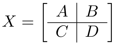
Each quadrant was transposed independently using our trans_4_4 kernel:

1. The upper-left matrix (in the image A) was transposed and stored at the same position.

2. The upper-right matrix (in the image B) was transposed and stored into the position originally occupied by the bottom-left matrix.

3. The bottom-left matrix (in the image C) would be transposed and stored into the position originally occupied by the upper-right matrix.

4. The bottom-right matrix (in the image D) was transposed and stored at the same position.

Transposing and swapping upper-right and bottom-left submatrices

    /*
    * Part 1.2:
    * Load 4x4 block of A (Left bottom, top right).
    */
    mov x4, x0 // A
    mov x5, x1 // B

    add x4, x4, #16
    add x5, x5, #16

    ldr q0, [x4]
    add x4, x4, x2
    ldr q1, [x4]
    add x4, x4, x2
    ldr q2, [x4]
    add x4, x4, x2
    ldr q3, [x4]

    // Right top
    mov x4, x0 // A
    mov x5, x1 // B

    add x4, x4, #128
    add x5, x5, #128
    
    ldr q12, [x4]
    add x4, x4, x2
    ldr q13, [x4]
    add x4, x4, x2
    ldr q14, [x4]
    add x4, x4, x2
    ldr q15, [x4]

    /*
    * Part 2.1:
    * Transpose 4x4 block.
    */
    // Left Bottom
    trn1 v4.4s, v0.4s, v2.4s
    trn1 v5.4s, v1.4s, v3.4s

    trn2 v6.4s, v0.4s, v2.4s
    trn2 v7.4s, v1.4s, v3.4s

    // Right Top
    trn1 v16.4s, v12.4s, v14.4s
    trn1 v17.4s, v13.4s, v15.4s

    trn2 v18.4s, v12.4s, v14.4s
    trn2 v19.4s, v13.4s, v15.4s

    /*
    * Part 2.2:
    * Transpose 4x4 block.
    */
    // Left Bottom
    zip1 v8.4s, v4.4s, v5.4s    
    zip1 v9.4s, v6.4s, v7.4s    

    zip2 v10.4s, v4.4s, v5.4s   
    zip2 v11.4s, v6.4s, v7.4s   

    // Right Top
    zip1 v20.4s, v16.4s, v17.4s 
    zip1 v21.4s, v18.4s, v19.4s 

    zip2 v22.4s, v16.4s, v17.4s 
    zip2 v23.4s, v18.4s, v19.4s

    /*
    * Part 3:
    * Store 4x4 block of Submatrix A''' into A''.
    */
    // Left Bottom (values from right top)
    mov x5, x1
    add x5, x5, #16

    str q20, [x5]
    add x5, x5, x3
    str q21, [x5]
    add x5, x5, x3
    str q22, [x5]
    add x5, x5, x3
    str q23, [x5]

    // Right top (values from left bottom)
    mov x5, x1
    add x5, x5, #128

    str q8, [x5]
    add x5, x5, x3
    str q9, [x5]
    add x5, x5, x3
    str q10, [x5]
    add x5, x5, x3
    str q11, [x5]

To optimize our initial implementation, we removed the PCS for all regsiters that we didn’t use. We also restructured our code for clarity and compactness.

Optimized second version of the transposition kernel

    mov x9, #2 // n loop

n_loop:

    mov x6, #2 // m loop

m_loop:
    /*
     * Part 1:
     * Transpose 4x4 block.
     */
    mov x7, x4
    mov x8, x5

    ldr q0, [x7]
    add x7, x7, x2

    ldr q1, [x7]
    add x7, x7, x2

    ldr q2, [x7]
    add x7, x7, x2

    ldr q3, [x7]

    /*
    * Part 2.1:
    * Transpose 4x4 block.
    */
    trn1 v4.4s, v0.4s, v2.4s
    trn1 v5.4s, v1.4s, v3.4s

    trn2 v6.4s, v0.4s, v2.4s
    trn2 v7.4s, v1.4s, v3.4s

    /*
    * Part 2.2:
    * Transpose 4x4 block.
    */
    zip1 v16.4s, v4.4s, v5.4s
    zip1 v17.4s, v6.4s, v7.4s

    zip2 v18.4s, v4.4s, v5.4s
    zip2 v19.4s, v6.4s, v7.4s

    /*
    * Part 3:
    * Store 4x4 block of A into B.
    */
    str q16, [x8]
    add x8, x8, x3

    str q17, [x8]
    add x8, x8, x3

    str q18, [x8]
    add x8, x8, x3

    str q19, [x8]

    // Jump 4 rows in A
    add x4, x4, x25

    // Jump 4 columns in B
    add x5, x5, x27

    sub x6, x6, #1
    cbnz x6, m_loop


    // Restore Pointer for A and B
    mov x4, x0
    mov x5, x1

    add x12, x12, x26
    add x13, x13, x25

    add x4, x4, x12
    add x5, x5, x13

    sub x9, x9, #1
    cbnz x9, n_loop

3.7.2 Performance Measuring

We measured the throughput of our transposition kernel in terms of memory transfer speed, since the core performance factor in this case is loading and storing elements efficiently.

trans_8_8 performance in GiB/s

Benchmarking trans_neon_8_8 performance ...
-----------------------------------------------
Measuring throughput for transposition in GiB/s
Total time (s):   1.26545
Data movements per Second:   8.09199e+10
Estimated GiB/s:   80.9199 GiB/s
-----------------------------------------------

Benchmarking v2_trans_neon_8_8 performance ...
-----------------------------------------------
Measuring throughput for transposition in GiB/s
Total time (s):   0.902975
Data movements per Second:   1.13403e+11
Estimated GiB/s:   113.403 GiB/s
-----------------------------------------------

Our benchmarking results show that the initial version achieved approximately 81 GiB/s. With our optimizations, we increased this to about 113 GiB/s.